
A Crash Course on Information Gain & some other DataMining terms and How To Get There
November 21, 2007 Posted by Emre S. Tasci
Suppose that you have -let’s say- 5 pipelines outputting Boolean values seemingly randomly such as:
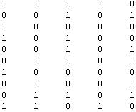
Now, we will be looking for a possible relation between these variables -let’s name that {a,b,c,d,e}� (Suppose that we do not know that the first 3 variables (a,b,c)� are randomly tossed, while the 4th (d)� is just “a AND b” and the 5th one (e) is actually “NOT a”).
- We look for different possible values of each variable and store them in an array called posVals (as obvius, from “Possible Values”). In our example, each of the variables can have only two values, so our posVals array will look something like this:

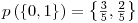
- Now that we know the possible outcomes for each of the variables, we calculate the probability of each of these values by simply counting them and then dividing to the total number of output. As an example, for the 3rd variable,� there are four 0’s and 6 1’s totaling 10 values. So, the probability of a chosen value to be 0 would be 4 out of 10 and 6/10 for 1. We store the probabilities in an array called probs this time which is like
�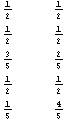
In the� 3rd row, the probabilities for the c variable are stored in the order presented in the posVals array (check the 3rd row of posVals to see that the first value is 1 and the second is 0). You can object the unnecessity of storing the second row of probs because, the second row is always equal to 1-probs[[1]] (I will be using the Mathematica notation for array elements, with a[[1]] meaning the 1st row if a is a matrix, or 1st element if a is a 1-D List; a[[1]][[3]] meaning the element on the first row and third column of the matrix a), but it is only a specific case that we are dealing with Boolean outputs. Yes,� a variable’s probability always equals to the sum of the probabilities of all the other variables subtracted from 1 but we will keep record of all the probabilities for practical reasons. - Now we will calculate the entropy for each variable. Entropy is a measure of order in a distribution and a higher entropy corresponds to a more disordered system. For our means, we will calculate the entropy as

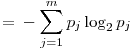
In these formulas, H represents the entropy, represents the probability of the jth value for variable X. Let’s store this values in the entropies array.
 - Special Conditional Entropy,
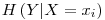 � is defined as the entropy of the Y variable values for which the corresponding X variable values equal to
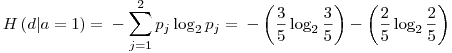
  .� For� our given example, let’s calculate H(d|a=1): Searching through the data, we see that, a=1 for rows: {1,3,4,7,10} and the values of d in these rows correspond to: {1,0,0,0,1}. Let’s assume this set ({1,0,0,0,1}) as a brand new set and go on from here.� Applying the definition of the entropy given in the 3rd step, we have:
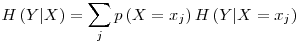
- Conditional Entropy,
 is the entropy including all the possible values of the variable being tested (X)� as having a relation to the� targeted� variable (Y). It is calculated as:
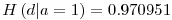
Again, if we look at our example, since we have H(d|a=1) =� 0.970951, p(a=1) = 0.5 ; and if we calculate H(d|a=0) in a similar way as in step 4, we find H(d|a=0) = 0 and taking
we find that H(d|a) = 0.5 x 0.970951 + 0.5 x 0 = 0.4854755 - Information Gain,
 – is a measure of the effect a variable (X)� is having against� a targetted variable (Y) with the information on the entropy of the targetted variable itself (H(Y))� taken into account. It is calculated as:

For our example , H(d) = 0.721928 and we calculated H(d|a=0) = 0.4854755 so, IG(d|a) = 0.236453. Summing up, for the data (of 10 for each variable)� presented in step 1, we have the Information Gain Table as:
| X |
IG(e|X) |
X |
IG(d|X) |
X |
IG(c|X) |
| a |
1.0 |
a |
0.236453 |
a |
0.124511 |
| b |
0.0290494 |
b |
0.236453 |
b |
0.0 |
| c |
0.124511 |
c |
0.00740339 |
d |
0.00740339 |
| d |
0.236453 |
e |
0.236453 |
e |
0.124511 |
| X |
IG(b|X) |
X |
IG(a|X) |
| a |
0.0290494 |
b |
0.0290494 |
| c |
0.0 |
c |
0.124511 |
| d |
0.236453 |
d |
0.236453 |
| e |
0.0290494 |
e |
1.0 |
And here are the results for 1000 values per variable instead of 10:
| X |
IG(e|X) |
X |
IG(d|X) |
X |
IG(c|X) |
| a |
0.996257 |
a |
0.327922 |
a |
0.000500799 |
| b |
0.000716169 |
b |
0.29628 |
b |
0.00224924 |
| c |
0.000500799 |
c |
0.000982332 |
d |
0.000982332 |
| d |
0.327922 |
e |
0.327922 |
e |
0.000500799 |
| X |
IG(b|X) |
X |
IG(a|X) |
| a |
0.000716169 |
b |
0.000716169 |
| c |
0.00224924 |
c |
0.000500799 |
| d |
0.29628 |
d |
0.327922 |
| e |
0.000716169 |
e |
0.996257 |
What can we say about the relationships from these Information Gain results?
- H(Y|X) = H(X|Y) – Is this valid for this specific case or is it valid for� general?
- Variable a: We can most probably guess a if we had known e, and it is somehow correlated with d.
- Variable b: It is correlated with d.
- Variable c: There doesn’t seem to be any correlation.
- Variable d: It is equally correlated with a&e and also correlated with b very closely to that correlation with a&e.
- Variable e: It is VERY strongly correlated with a and� it is somehow correlated with d.
Let’s take it on from here, with the variable d:
This is the IG table for 10000 data per each variable:
| X |
IG(d|X) |
| a |
0.30458 |
| b |
0.297394 |
| c |
0.00014876 |
| e |
0.30458 |
This is the IG table for 100000 data per each variable:
| X |
IG(d|X) |
| a |
0.309947 |
| b |
0.309937 |
| c |
1.97347×10^-6 |
| e |
0.309947 |
You can download the Mathematica sheet for this example : Information Gain Example
You will also need the two libraries (Matrix & DataMining) to run the example.

November 22, 2007 at 2:01 pm
If you run the example code, you will see that you are receving different values from the results presented here, even if you use the same 10 data. This is because of the definition of the entropy. In the entry, I’m using the binary entropy with Log base 2, but in the Mathematica functions I’ve posted, I switched the Log base to e for general purposes.
You can easily switch back to the former version by simply changing the line in the definition of the function DMEntropyEST from
Return[-Sum[problist[[i]] Log[problist[[i]]], {i,
Length[problist]}]];
to
Return[-Sum[problist[[i]] Log[2,problist[[i]]], {i, Length[problist]}]];
in the DataMining Functions Library file “estrefdm.nb”
April 7, 2008 at 4:22 pm
[…] theoretical background and mathematica version of the functions refer to : A Crash Course on Information Gain & some other DataMining terms and How To Get There (my 21/11/2007dated […]