
Quantum Espresso meets bash : Automated running for various values
March 13, 2012 Posted by Emre S. Tasci
Now that we can include comments in our input files and submit our jobs in a tidied up way, it’s time to automatize the “convergence search” process. For this, we’ll be using the same diamond example of the previous entry.
Suppose that we want to calculate the energies corresponding to various values of the lattice parameter a, ranging from 3.2 to 4, incrementing by 2: 3.2, 3.4, … , 4.0
Incrementation:
In bash, you can define a for loop to handle this:
for (( i = 1; i <= 9; i++ ))
do
  echo $i;
done

1
2
3
4
5
6
7
8
9
But to work with rational numbers, things get a little bit complex:
for (( i = 1; i <= 5; i++ ))
do
    val=$(awk "BEGIN {print 3+$i/5 }")
    echo $val;
done

3.2
3.4
3.6
3.8
4
Alas, it is still not very practical to everytime calculate the necessary values to produce our intended range. This is where the mighty Octave once again comes to the rescue: [A:I:B] in Octave defines a range that starts from A, and continues by incrementing by I until B is reached (or exceeded). So, here is our example in Octave:
octave:1> [3.2:0.2:4]
ans =

   3.2000   3.4000   3.6000   3.8000   4.0000
You can generate temporary input scripts for Octave but better yet, you can also feed simple scripts directly to Octave:
sururi@husniya:~/shared/qe/diamond_tutorial$ echo "[3.2:0.2:4]"|octave -q
ans =

   3.2000   3.4000   3.6000   3.8000   4.0000
The “-q” parameter causes Octave to run in “quiet” mode, so we just feed the range via pipe to Octave and will harvest the output. In general, we’d like to keep the “ans =” and the blank lines out, and then, when there are more than 1 line’s worth of output, Octave puts the “Column” information as in:
octave:4> [3:0.1:4]
ans =

 Columns 1 through 9:

   3.0000   3.1000   3.2000   3.3000   3.4000   3.5000   3.6000   3.7000   3.8000

 Columns 10 and 11:

   3.9000   4.0000
all these nuisances can go away via a simple “grep -v” (with the ‘v’ parameter inverting the filter criteria):
sururi@vala:/tmp$ echo "[3.2:0.1:4]"|octave -q|sed -n "2,1000p"| grep -v "Column"

   3.2000   3.3000   3.4000   3.5000   3.6000   3.7000   3.8000   3.9000

   4.0000

sururi@vala:/tmp$ echo "[3.2:0.1:4]"|octave -q|sed -n "2,1000p"| grep -v "Column"|grep -v -e "^$"
   3.2000   3.3000   3.4000   3.5000   3.6000   3.7000   3.8000   3.9000
   4.0000
Replacement:
Now that we have the variable’s changing values, how are we gonna implement it to the input script? By search and replace. Suppose, we have a template in which the variable’s value is specified by “#REPLACE#”, all we need to do is to “sed” the file:
cat diamond.scf.in | sed "s:#REPLACE#:$a:g">tmp_$a.in
where “$a” is the current value in the iteration.
Parsing the Energy:
We submit this job via mpirun (in our case via mpi-pw.x of the previous post) and parse the output for the final energy:
grep -e ! tmp_$a.out|tail -n1|awk '{print $(NF-1)}'For each iteration we thus obtain the energy for our $a value, so we put them together in two columns into a data file I’d like to call “E_vs_$a.txt”.
The Script:
Putting all these together, here is the script in its full glory:
#!/bin/bash

# Takes in the template Quantum Espresso input file, runs it iteratively
# changing the #REPLACE# parameters iteratively with the range elements,
# grepping the energy and putting it along with the current value of the
# #REPLACE# parameter.
#
# Emre S. Tasci, 03/2012

# Example: Suppose that the file "diamond.scf.in" contains the following line:
#   A = #REPLACE#
# Calling "qe-opti.sh diamond.scf.in a 3.2 0.2 4.2" would cause that line to be modified as
#   A = 3.2
# and submitted, followed by
#   A = 3.4, 3.6, .., 4.2 in the sequential runs.
#
# at the end, having constructed the E_vs_a.txt file.

if [ $# -ne 5 ]
then
    echo "Usage: qe-opti.sh infile_template.in variable_name initial_value increment     final_value"
    echo "Example: qe-opti.sh diamond.scf.in a 3.2 0.2 4.2"
    echo -e "\nNeeds octave to be accessible via \"octave\" command for the range to     work"
    echo -e "\nEmre S. Tasci, 03/2012"
    exit
fi

logext=".txt"
logfilename=E_vs_$2$logext
rm -f $logfilename

range=$(echo "[$3:$4:$5]"|octave -q|sed -n "2,1000p"|grep -vr "^$"|grep -v "Column")
for a in $range
do
    # echo $a
    cat $1|sed "s:#REPLACE#:$a:g">tmp_$a.in
    /home/sururi/bin/mpi-pw.x 4 tmp_$a.in
energ=$(grep -e ! tmp_$a.out|tail -n1|awk '{print $(NF-1)}')
    # echo $energ
    echo -e $a "    " $energ >> $logfilename
    echo -e $a "    " $energ
done

echo "Results stored in: "$logfilename
Action:
Modify the sample input from the previous post so that it’s lattice parameter A is designated as something like “A = #REPLACE#”, as in:
sururi@bebop:~/shared/qe/diamond_tutorial$ grep "REPLACE" -B2 -A2 diamond.scf.in
    # a,b,c in Angstrom =======
    #A = 3.56712
    A = #REPLACE#
    B = 2.49
    C = 2.49
Then call the qe-opti.sh script with the related parameters:
sururi@bebop:~/shared/qe/diamond_tutorial$ qe-opti.sh diamond.scf.in a 3.2 0.2 4.2
Running: mpirun -n 4 /usr/share/espresso-4.3.2/bin/pw.x < tmp_3.2000.in > tmp_3.2000.out

Start : Tue Mar 13 23:21:07 CET 2012
Finish: Tue Mar 13 23:21:08 CET 2012
Elapsed time:0:00:01

3.2000      -22.55859979
Running: mpirun -n 4 /usr/share/espresso-4.3.2/bin/pw.x < tmp_3.4000.in > tmp_3.4000.out

Start : Tue Mar 13 23:21:08 CET 2012
Finish: Tue Mar 13 23:21:09 CET 2012
Elapsed time:0:00:01

3.4000      -22.67717405
Running: mpirun -n 4 /usr/share/espresso-4.3.2/bin/pw.x < tmp_3.6000.in > tmp_3.6000.out

Start : Tue Mar 13 23:21:09 CET 2012
Finish: Tue Mar 13 23:21:10 CET 2012
Elapsed time:0:00:01

3.6000      -22.69824702
Running: mpirun -n 4 /usr/share/espresso-4.3.2/bin/pw.x < tmp_3.8000.in > tmp_3.8000.out

Start : Tue Mar 13 23:21:10 CET 2012
Finish: Tue Mar 13 23:21:11 CET 2012
Elapsed time:0:00:01

3.8000      -22.65805473
Running: mpirun -n 4 /usr/share/espresso-4.3.2/bin/pw.x < tmp_4.0000.in > tmp_4.0000.out

Start : Tue Mar 13 23:21:11 CET 2012
Finish: Tue Mar 13 23:21:13 CET 2012
Elapsed time:0:00:02

4.0000      -22.57776354
Running: mpirun -n 4 /usr/share/espresso-4.3.2/bin/pw.x < tmp_4.2000.in > tmp_4.2000.out

Start : Tue Mar 13 23:21:13 CET 2012
Finish: Tue Mar 13 23:21:14 CET 2012
Elapsed time:0:00:01

4.2000      -22.47538891
Results stored in: E_vs_a.txt
Where the “E_vs_a.txt” contains the … E vs a values!:
sururi@bebop:~/shared/qe/diamond_tutorial$ cat E_vs_a.txt
3.2000      -22.55859979
3.4000      -22.67717405
3.6000      -22.69824702
3.8000      -22.65805473
4.0000      -22.57776354
4.2000      -22.47538891
You can easily plot it using GNUPlot or whatever you want. In my case, I prefer GNUPlot:
sururi@husniya:~/shared/qe/diamond_tutorial$ plot E_vs_a.txt
giving me:

Other than the ‘plot’, I’ve also written another one, fit for data sets just like these where you have a parabol-like data and you’d like to try fitting it and here is what it does (automatically):
sururi@husniya:~/shared/qe/diamond_tutorial$ plotfitparabol.sh E_vs_a.txt
func    f(x)=0.674197*x*x-4.881275*x-13.855234
min, f(min)    3.620066 -22.690502

Here are the source codes of the ‘plot’ and ‘plotfitparabol.sh’ scripts. Doei!
sururi@mois:/vala/bin$ cat plot
#!/bin/bash
gnuplot -persist <<END
set term postscript enhanced color
set output "$1.ps"
plot "$1" $2 $3

set term wxt
replot
END
sururi@mois:/vala/bin$ cat plotfitparabol.sh
#!/bin/bash

# Usage : plotfitparabol.sh <datafile>

# Reads the data points from the given file
# then uses Octave's "polyfit" function to calculate the coefficients
# for the quadratic fit and also the minimum (maximum) value.
# Afterwards, prepares a GNUPlot script to display:
#    the data set (scatter)
#    fit function
#    the extremum point's value
#
# Written with Quantum Espresso optimizing procedures in mind.


if [ $# -ne 1 ]
then
    echo "Usage: plotfitparabol.sh <datafile>"
    echo "Example: plotfitparabol.sh E_vs_A.txt"
    echo -e "\nNeeds octave to be accessible via \"octave\" command to work"
    echo -e "\nEmre S. Tasci <emre.tasci@ehu.es>, 03/2012"
    exit
fi

octave_script="data=load(\"$1\");m=polyfit(data(:,1),data(:,2),2);min=-m(2)*0.5/m(1);fmin=min*min*m(1)+min*m(2)+m(3);printf(\"f(x)=%f*x*x%+f*x%+f|%f\t%f\",m(1),m(2),m(3),min,fmin)"
oct=$(echo $octave_script|octave -q)
#echo $oct

func=${oct/|*/ }
minfmin=${oct/*|/ }
echo -e "func \t" $func
echo -e "min, f(min) \t" $minfmin

echo '$func
set term postscript enhanced color
set label "$1" at graph 0.03, graph 0.94
set output "$1.ps"
plot "$1" title "data", f(x) title "$func", "<echo '$minfmin'" title "$minfmin"

set term wxt
replot'

gnuplot -persist <<END
$func
set term postscript enhanced color
set label "$1" at graph 0.03, graph 0.94
set output "$1.ps"
plot "$1" title "data", f(x) title "$func", "<echo '$minfmin'" title "$minfmin"

set term wxt
replot
END
Coordination Numbers
September 3, 2009 Posted by Emre S. Tasci
Recently, we are working on liquid alloys and for our work, we need the coordination number distribution. It’s kind of a gray area when you talk about coordination number of atoms in a liquid but it’s better than nothing to understand the properties and even more. I’d like to write a log on the tools I’ve recently coded/used in order to refer to in the future if a similar situation occurs. Also, maybe there are some others conducting similar research so, the tools introduced here may be helpful to them.
Recently, while searching recent publications on liquid alloys, I’ve found a very good and resourceful article on liquid Na-K alloys by Dr. J.-F. Wax (“Molecular dynamics study of the static structure of liquid Na-K alloys”, Physica B 403 (2008) 4241-48 | doi:10.1016/j.physb.2008.09.014). In this paper, among other properties, he had also presented the partial pair distribution functions. Partial-pair distribution functions is the averaged probability that you’ll encounter an atom in r distance starting from another atom. In solid phase, due to the symmetry of the crystal structure, you have discrete values instead of a continuous distribution and everything is crystal clear but I guess that’s the price we pay dealing with liquids. 8)
Partial-pair distribution functions are very useful in the sense that they let you derive the bond-length between constituent atom species, corresponding to the first minimums of the plots. Hence, one can see the neighborhood ranges by just looking at the plots.
I’ve sent a mail to Dr. Wax explaining my research topics and my interest and asking for his research data to which he very kindly and generously replied by providing his data.
He had sent me a big file with numerous configurations (coordinates of the atoms) following each other. The first -and the simplest- task was to split the file into seperate configuration files via this bash script:
#!/bin/bash
# Script Name: split_POS4.sh
# Splits the NaK conf files compilation POS4_DAT into sepearate
# conf files.
# Emre S. Tasci <e.tasci@tudelft.nl>
#                                              01/09/09

linestart=2
p="p"
for (( i = 1; i <= 1000; i++ ))
do
    echo $i;
    lineend=$(expr $linestart + 2047)
    confname=$(printf "%04d" $i)
    echo -e "3\n2048" > $confname
    sed -n "$linestart,$(echo $lineend$p)" POS4_DAT >> $confname
    linestart=$(expr $lineend + 1)
    cat $confname | qhull i TO $confname.hull
done
(The compilation was of 1000 configurations, each with 2048 atoms)
As you can check in the line before the “done” closer, I’ve -proudly- used Qhull software to calculate the convex hull of each configuration. A convex hull is the -hopefully minimum- shape that covers all your system. So, for each configuration I now had 2 files: “xxxx” (where xxxx is the id/number of the configuration set) storing the coordinates (preceded by 3 and 2048, corresponding to dimension and number of atoms information for the qhull to parse & process) and “xxxx.hull” file, generated by the qhull, containing the vertices list of each facet (preceded by the total number of facets).
A facet is (in 3D) the plane formed by the vertice points. Imagine a cube, where an atom lies at each corner, 3 in the inside. So, we can say that our system consists of 11 atoms and the minimal shape that has edges selected from system’s atoms and covering the whole is a cube, with the edges being the 8 atoms at the corners. Now, add an atom floating over the face at the top. Now the convex hull that wraps our new system would no longer be a 6-faced, 8-edged cube but a 9-faced, 9-edged polygon. I need to know the convex hull geometry in order to correctly calculate the coordination number distributions (details will follow shortly).
The aforementioned two files look like:
sururi@husniya hull_calcs $ head 0001
3
2048
 0.95278770E+00 0.13334565E+02 0.13376155E+02
 0.13025256E+02 0.87618381E+00 0.20168993E+01
 0.12745038E+01 0.14068998E-01 0.22887323E+01
 0.13066590E+02 0.20788591E+01 0.58119183E+01
 0.10468218E+00 0.58523640E-01 0.64288678E+01
 0.12839412E+02 0.13117012E+02 0.79093881E+01
 0.11918105E+01 0.12163854E+02 0.10270868E+02
 0.12673985E+02 0.11642538E+02 0.10514597E+02
sururi@husniya hull_calcs $ head 0001.hull
180
568 1127 1776
1992 104 1551
956 449 1026
632 391 1026
391 632 1543
391 956 1026
966 632 1026
966 15 1039
632 966 1039
The sets of 3 numbers in the xxxx.hull file is the ids/numbers of the atoms forming the edges of the facets, i.e., they are the vertices.
To calculate the coordination number distribution, you need to pick each atom and then simply count the other atoms within the cut-off distance depending on your atom’s and the neighboring atom’s species. After you do the counting for every atom, you average the results and voilà ! there is your CN distribution. But here’s the catch: In order to be able to count properly, you must make sure that, your reference atom’s cutoff radii stay within your system — otherwise you’ll be undercounting. Suppose your reference atom is one of the atoms at the corners of the cube: It will (generally/approximately) lack 7/8 of the neighbouring atoms it would normally have if it was to be the center atom of the specimen/sample. Remember that we are studying a continuous liquid and trying to model the system via ensembles of samples. So we should omit these atoms which has neighborhoods outside of our systems. Since neighborhoods are defined through bond-length, we should only include the atoms with a distance to the outside of at least cut-off radii. The “outside” is defined as the region outside the convex hull and it’s designated by the facets (planes).
From the xxxx.hull file, we have the ids of the vertice atoms and their coordinates are stored in the xxxx file. To define the plane equation

we will use the three vertice points, say p1, p2 and p3. From these 3 points, we calculate the normal n as:
\times\left(\vec{p_3}-\vec{p_1}\right)")
then, the plane equation (hence the coefficients a,b,c,d) can be derived by comparing the following equation:
+n_{y}\left(y-y_{0} \right)+n_{z}\left(z-z_{0} \right) = 0")
Here, (x0,y0,z0) are just the coordinates of any of the vertice points. And finally, the distance D between a point p1(x1,y1,z1) and a plane (a,b,c,d) is given by:

Since vector operations are involved, I thought it’s better to do this job in Octave and wrote the following script that calculates the coefficients of the facets and then sets down to find out the points whose distances to all the facets are greater than the given cut-off radius:
sururi@husniya trunk $ cat octave_find_atoms_within.m
DummyA = 3;
%conf_index=292;

% Call from the command line like :
%   octave -q --eval "Rcut=1.65;conf_index=293;path='$(pwd)';" octave_find_atoms_within.m
% hence specifying the conf_index at the command line.

% Emre S. Tasci <e.tasci@tudelft.nl>                    *
%
% From the positions and vertices file, calculates the plane
% equations (stored in "facet_coefficients") and then
% filters the atoms with respect to their distances to these
% facets. Writes the output to
% "hull_calcs/xxxx_insiders.txt" file
%                                              03/09/09 */

conf_index_name = num2str(sprintf("%04d",conf_index));;
%clock
clear facet_coefficients;
facet_coefficients = [];
global p v facet_coefficients
fp = fopen(strcat(path,"/hull_calcs/",conf_index_name));
k = fscanf(fp,"%d",2); % 1st is dim (=3), 2nd is number of atoms (=2048)
p = fscanf(fp,"%f",[k(1),k(2)]);
p = p';
fclose(fp);
%p = load("/tmp/del/delco");
fp = fopen(strcat(path,"/hull_calcs/",conf_index_name,".hull"));
k = fscanf(fp,"%d",1);% number of facets
v = fscanf(fp,"%d",[3,k]);
v = v';
fclose(fp);
%v = load("/tmp/del/delver");

function [a,b,c,d,e] = getPlaneCoefficients(facet_index)
    global p v
    % Get the 3 vertices
    p1 = p(v(facet_index,1)+1,:); % The +1s come from the fact
    p2 = p(v(facet_index,2)+1,:); % that qhull enumeration begins
    p3 = p(v(facet_index,3)+1,:); % from 0 while Octave's from 1

    %printf("%d: %f %f %f %f %f %f %f %f %f\n",facet_index,p1,p2,p3);

    % Calculate the normal
    n = cross((p2-p1),(p3-p1));

    % Calculate the coefficients of the plane :
    % ax + by + cz +d = 0
    a = n(1);
    b = n(2);
    c = n(3);
    d = -(dot(n,p1));
    e = norm(n);
    if(e==0)
        printf("%f\n",p1);
        printf("%f\n",p2);
        printf("%f\n",p3);
        printf("%d\n",facet_index);
    endif
endfunction

function dist = distanceToPlane(point_index,facet_index)
    global p facet_coefficients
    k = facet_coefficients(facet_index,:);
    n = [k(1) k(2) k(3)];
    dist = abs(dot(n,p(point_index,:)) + k(4)) / k(5);
endfunction

for i = [1:size(v)(1)]
    [a,b,c,d,e] = getPlaneCoefficients(i);
    facet_coefficients = [ facet_coefficients ; [a,b,c,d,e]];
endfor

%Rcut = 1.65; % Defined from command line calling
% Find the points that are not closer than Rcut
inside_atoms = [];
for point = [1:size(p)(1)]
%for point = [1:100]
    inside=true;
    for facet = [1:size(v)(1)]
    %for facet = [1:10]
        %printf("%d - %d : %f\n",point,facet,dist);
        if (distanceToPlane(point,facet)<Rcut)
            inside = false;
            break;
        endif
    endfor
    if(inside)
        inside_atoms = [inside_atoms point-1];
    endif
endfor

fp = fopen(strcat(path,"/hull_calcs/",conf_index_name,"_insiders.txt"),"w");
fprintf(fp,"%d\n",inside_atoms);
fclose(fp);
%clock
This script is runned within the following php code which then takes the filtered atoms and does the counting using them:
<?PHP
/* Emre S. Tasci <e.tasci@tudelft.nl>                    *
 *
 * parse_configuration_data.php
 *
 * Written in order to parse the configuation files
 * obtained from J.F. Wax in order to calculate the
 * Coordination Number distribution. Each configuration
 * file contain 2048 atoms' coordinates starting at the
 * 3rd line. There is also a convex hull file generated
 * using qhull (http://www.qhull.com) that contains the
 * indexes (starting from 0) of the atoms that form the
 * vertices of the convex hull. Finally there is the
 * IP.dat file that identifies each atom (-1 for K; 1 for
 * Na -- the second column is the relative masses).
 *
 *                                              02/09/09 */

/*
# if present, remove the previous run's results file
if(file_exists("results.txt"))
    unlink("results.txt");
 */

error_reporting(E_ALL ^ E_NOTICE);

if(!file_exists("results.txt"))
{
    $fp = fopen("results.txt","w");
    fwrite($fp,"CONF#"."\tNa".implode("\tNa",range(1,20))."\tK".implode("\tK",range(1,20))."\n");
    fclose($fp);
}

# Support for command line variable passing:
for($i=1;$i<sizeof($_SERVER["argv"]);$i++)
{
        list($var0,$val0) = explode("=",$_SERVER["argv"][$i]);
        $_GET[$var0] = $val0;
}

if($_GET["configuration"])
    calculate($_GET["configuration"]);
else
    exit("Please specify a configuration number [php parse_configuration_data.php configuration=xxx]\n");

function calculate($conf_index)
{
    # Define the atoms array
    $arr_atoms = Array();

    # Get the information from the files
    parse_types($arr_atoms);
    $refs = get_vertices($conf_index);
    parse_coordinates($arr_atoms,$conf_index);

    # Define the Rcut-off values (obtained from partial parid distribution minimums)
    $Rcut_arr = Array();
    $Rscale = 3.828; # To convert reduced distances to Angstrom (if needed)
    $Rscale = 1; # To convert reduced distances to Angstrom
    $Rcut_arr["Na"]["Na"] = 1.38 * $Rscale;
    $Rcut_arr["Na"]["K"]  = 1.65 * $Rscale;
    $Rcut_arr["K"]["Na"]  = 1.65 * $Rscale;
    $Rcut_arr["K"]["K"]   = 1.52 * $Rscale;
    $Rcut = $Rcut_arr["Na"]["K"]; # Taking the maximum one as the Rcut for safety

    /*
    # We have everything we need, so proceed to check
    # if an atom is at safe distance wrt to the vertices

    # Define all the ids
    $arr_test_ids = range(0,2047);
    # Subtract the ref atoms' ids
    $arr_test_ids = array_diff($arr_test_ids, $refs);
    sort($arr_test_ids);
    //print_r($arr_test_ids);

    $arr_passed_atom_ids = Array();
    # Check each atom against refs
    for($id=0, $size=sizeof($arr_test_ids); $id<$size; $id++)
    {
        //echo $id."\n";
        $arr_atoms[$arr_test_ids[$id]]["in"] = TRUE;
        foreach ($refs as $ref)
        {
            $distance = distance($arr_atoms[$arr_test_ids[$id]],$arr_atoms[$ref]);
            //echo "\t".$ref."\t".$distance."\n";
            if($distance < $Rcut)
            {
                $arr_atoms[$arr_test_ids[$id]]["in"] = FALSE;
                break;
            }
        }
        if($arr_atoms[$arr_test_ids[$id]]["in"] == TRUE)
            $arr_passed_atom_ids[] = $arr_test_ids[$id];
    }
     */

    # Run the octave script file to calculate the inside atoms
    if(!file_exists("hull_calcs/".sprintf("%04d",$conf_index)."_insiders.txt"))
    exec("octave -q --eval \"Rcut=".$Rcut.";conf_index=".$conf_index.";path='$(pwd)';\" octave_find_atoms_within.m");

    # Read the file generated by Octave
    $arr_passed_atom_ids = file("hull_calcs/".sprintf("%04d",$conf_index)."_insiders.txt",FILE_IGNORE_NEW_LINES);

    $arr_test_ids = range(0,2047);
    $arr_test_ids = array_diff($arr_test_ids, $refs);
    sort($arr_test_ids);
    for($i=0, $size=sizeof($arr_test_ids);$i<$size;$i++)
        $arr_atoms[$arr_test_ids[$i]]["in"]=FALSE;

    # Begin checking every passed atom
    foreach($arr_passed_atom_ids as $passed_atom_id)
    {
        $arr_atoms[$passed_atom_id]["in"] = TRUE;
        for($i=0, $size=sizeof($arr_atoms); $i<$size; $i++)
        {
            $distance = distance($arr_atoms[$passed_atom_id],$arr_atoms[$i]);
            //echo $passed_atom_id."\t---\t".$i."\n";
            if($distance < $Rcut_arr[$arr_atoms[$passed_atom_id]["id"]][$arr_atoms[$i]["id"]] && $distance>0.001)
                $arr_atoms[$passed_atom_id]["neighbour_count"] += 1;
        }
    }

    # Do the binning
    $CN_Na = Array();
    $CN_K  = Array();
    for($i=0, $size=sizeof($arr_atoms); $i<$size; $i++)
    {
        if(array_key_exists("neighbour_count",$arr_atoms[$i]))
        {
            ${"CN_".$arr_atoms[$i]['id']}[$arr_atoms[$i]["neighbour_count"]] += 1;
        }
    }

    ksort($CN_Na);
    ksort($CN_K);

    //print_r($arr_atoms);
    //print_r($CN_Na);
    //print_r($CN_K);

    # Report the results
    $filename = "results/".sprintf("%04d",$conf_index)."_results.txt";
    $fp = fopen($filename,"w");
    fwrite($fp, "### Atoms array ###\n");
    fwrite($fp,var_export($arr_atoms,TRUE)."\n");
    fwrite($fp, "\n### CN Distribution for Na ###\n");
    fwrite($fp,var_export($CN_Na,TRUE)."\n");
    fwrite($fp, "\n### CN Distribution for K ###\n");
    fwrite($fp,var_export($CN_K,TRUE)."\n");

    # Percentage calculation:
    $sum_Na = array_sum($CN_Na);
    $sum_K  = array_sum($CN_K);
    foreach($CN_Na as $key=>$value)
        $CN_Na[$key] = $value * 100 / $sum_Na;
    foreach($CN_K  as $key=>$value)
        $CN_K[$key]  = $value * 100 / $sum_K;
    //print_r($CN_Na);
    //print_r($CN_K);
    fwrite($fp, "\n### CN Distribution (Percentage) for Na ###\n");
    fwrite($fp,var_export($CN_Na,TRUE)."\n");
    fwrite($fp, "\n### CN Distribution (Percentage) for K ###\n");
    fwrite($fp,var_export($CN_K,TRUE)."\n");
    fclose($fp);

    # Write the summary to the results file
    $fp = fopen("results.txt","a");
    for($i=1;$i<=20;$i++)
    {
        if(!array_key_exists($i,$CN_Na))
            $CN_Na[$i] = 0;
        if(!array_key_exists($i,$CN_K))
            $CN_K[$i] = 0;
    }
    ksort($CN_Na);
    ksort($CN_K);
    fwrite($fp,sprintf("%04d",$conf_index)."\t".implode("\t",$CN_Na)."\t".implode("\t",$CN_K)."\n");
    fclose($fp);

}

function parse_types(&$arr_atoms)
{
    # Parse the types
    $i = 0;
    $fp = fopen("IP.DAT", "r");
    while(!feof($fp))
    {
        $line = fgets($fp,4096);
        $auxarr = explode(" ",$line);
        if($auxarr[0]==-1)
            $arr_atoms[$i]["id"] = "Na";
        else
            $arr_atoms[$i]["id"] = "K";
        $i++;
    }
    fclose($fp);
    array_pop($arr_atoms);
    return 0;
}

function get_vertices($conf_index)
{
    $arr_refs = Array();

    # Get the ids of the vertices of the convex hull
    $filename = "hull_calcs/".sprintf("%04d",$conf_index).".hull";
    $fp = fopen($filename, "r");

    # Bypass the first line
    $line = fgets($fp,4096);

    while(!feof($fp))
    {
        $line = fgets($fp,4096);
        $auxarr = explode(" ",$line);
        array_pop($auxarr);
        $arr_refs = array_merge($arr_refs, $auxarr);
    }
    fclose($fp);
    // $arr_refs = array_unique($arr_refs); # This doesn't lose the keys
    $arr_refs = array_keys(array_count_values($arr_refs)); # But this does.
    return $arr_refs;
}

function parse_coordinates(&$arr_atoms, $conf_index)
{
    # Parse the coordinates
    $i = 0;
    $filename = "hull_calcs/".sprintf("%04d",$conf_index);
    $fp = fopen($filename, "r");

    # Bypass the first two lines
    $line = fgets($fp,4096);
    $line = fgets($fp,4096);

    while(!feof($fp))
    {
        $line = fgets($fp,4096);
        $arr_atoms[$i]["coords"] = explode(" ",$line);
        array_shift($arr_atoms[$i]["coords"]);
        $i++;
    }
    fclose($fp);
    array_pop($arr_atoms);
    return 0;
}

function distance(&$atom1,&$atom2)
{
    # Calculate the distance between the two atoms
    $x1 = $atom1["coords"][0];
    $x2 = $atom2["coords"][0];
    $y1 = $atom1["coords"][1];
    $y2 = $atom2["coords"][1];
    $z1 = $atom1["coords"][2];
    $z2 = $atom2["coords"][2];
    return sqrt(pow($x1-$x2,2) + pow($y1-$y2,2) + pow($z1-$z2,2));
}

?>
The code above generates a “results/xxxx_results.txt” file containing all the information obtained in arrays format and also appends to “results.txt” file the relevant configuration file’s CN distribution summary. The systems can be visualized using the output generated by the following plotter.php script:
<?PHP
/* Emre S. Tasci <e.tasci@tudelft.nl>                    *
 * Parses the results/xxxx_results.txt file and generates
 * an XYZ file such that the atoms are labeled as the
 * vertice atoms, close-vertice atoms and inside atoms..
 *                                              02/09/09 */

# Support for command line variable passing:
for($i=1;$i<sizeof($_SERVER["argv"]);$i++)
{
        list($var0,$val0) = explode("=",$_SERVER["argv"][$i]);
        $_GET[$var0] = $val0;
}

if($_GET["configuration"])
    $conf_index = $_GET["configuration"];
else
    exit("Please specify a configuration number [php plotter.php configuration=xxx]\n");

$filename = sprintf("%04d",$conf_index);

# Get the atom array from the results file. Since results file
# contains other arrays as well, we slice the file using sed for the
# relevant part
$last_arr_line = exec('grep "### CN Distribution" results/'.$filename.'_results.txt -n -m1|sed "s:^\([0-9]\+\).*:\1:gi"');
exec('sed -n "2,'.($last_arr_line-1).'p" results/'.$filename.'_results.txt > system_tmp_array_dump_file');
$str=file_get_contents('system_tmp_array_dump_file');
$atom_arr=eval('return '.$str.';');
unlink('system_tmp_array_dump_file');

# Now that we have the coordinates, we itarate over the atoms to check
# the characteristic and designate them in the XYZ file.
$fp = fopen("system_".$filename.".xyz","w");
fwrite($fp,sizeof($atom_arr)."\n");
fwrite($fp,"Generated by plotter.php\n");
for($i=0, $size=sizeof($atom_arr);$i<$size;$i++)
{
    if(!array_key_exists("in",$atom_arr[$i]))
        $atomlabel = "Mg";#Vertices
    elseif($atom_arr[$i]["in"]==TRUE)
        $atomlabel = $atom_arr[$i]["id"];#Inside atoms
    else
        $atomlabel = "O";#Close-vertice atoms
    fwrite($fp,$atomlabel."\t".implode("\t",$atom_arr[$i]["coords"]));
}
fclose($fp);
?>
which generates a “system_xxxx.xyz” file, ready to be viewed in a standard molecule viewing software. It designates the vertice atoms (of the convex hull, remember? 8)as “Mg” and the atoms close to them as “O” for easy-viewing purpose. A sample parsed file looks like this:

The filtered case of a sample Na-K system
The big orange atoms are the omitted vertice atoms; the small red ones are the atoms critically close to the facets and hence also omitted ones. You can see the purple and yellow atoms which have passed the test sitting happilly inside, with the counting done using them.. 8)
Some unit cell functions for Octave
May 23, 2009 Posted by Emre S. Tasci
I’ve written some functions to aid in checking the transformations as well as switching between the parameter â vector representations.
latpar2vec([a,b,c,alpha,beta,gamma])
Given the a,b,c,α,β and γ, the function calculates the lattice vectors
function f=latpar2vec(X)
% function f=latpar2vec([a,b,c,alpha,beta,gamma])
% Calculates the lattice vectors from the given lattice paramaters.

a     = X(1);
b     = X(2);
c     = X(3);
alpha = X(4);
beta  = X(5);
gamma = X(6);

% Converting the angles to radians:
alpha = d2r(alpha);
beta  = d2r(beta);
gamma = d2r(gamma);

%Aligning a with the x axis:
ax = a;
ay = 0;
az = 0;

%Orienting b to lie on the x-y plane:
bz = 0;

% Now we have 6 unknowns for 6 equations..
bx = b*cos(gamma);
by = (b**2-bx**2)**.5;
cx = c*cos(beta);
cy = (b*c*cos(alpha)-bx*cx)/by;
cz = (c**2-cx**2-cy**2)**.5;
f=[ax ay az
   bx by bz
   cx cy cz];
endfunction
latvec2par([ax ay az; bx by bz; cx cy cz])
Calculates the lattice parameters a,b,c,α,β and γ from the lattice vectors
function f=latvec2par(x)
% function f=latvec2par(x)
%     ax ay az
% x = bx by bz
%     cx cy cz
%
% takes the unit cell vectors and calculates the lattice parameters
% Emre S. Tasci <e.tasci@tudelft.nl>   03/10/08

av = x(1,:);
bv = x(2,:);
cv = x(3,:);

a = norm(av);
b = norm(bv);
c = norm(cv);

alpha = acos((bv*cv')/(b*c))*180/pi;
beta  = acos((av*cv')/(a*c))*180/pi;
gamma = acos((av*bv')/(a*b))*180/pi;

f = [a b c alpha beta gamma];
endfunction
volcell([a,b,c,A,B,G])
Calculates the volume of the cell from the given lattice parameters, which is the determinant of the matrice build from the lattice vectors.
function f=volcell(X)
% function f=volcell([a,b,c,A,B,G])
% Calculate the cell volume from lattice parameters
%
% Emre S. Tasci, 09/2008
a=X(1);
b=X(2);
c=X(3);
A=X(4); % alpha
B=X(5); % beta
G=X(6); % gamma
 f=a*b*c*(1-cos(d2r(A))^2-cos(d2r(B))^2-cos(d2r(G))^2+2*cos(d2r(A))*cos(d2r(B))*cos(d2r(G)))^.5;
endfunction
Why’s there no “volcell” function for the unit cell vectors? You’re joking, right? (det(vector)) ! 🙂
Example
octave:13> % Define the unit cell for PtSn4 :
octave:13> A = latpar2vec([ 6.41900 11.35700  6.38800  90.0000  90.0000  90.0000 ])
A =

    6.41900    0.00000    0.00000
    0.00000   11.35700    0.00000
    0.00000    0.00000    6.38800

octave:14> % Cell volume :
octave:14> Apar = [ 6.41900 11.35700  6.38800  90.0000  90.0000  90.0000 ]
Apar =

    6.4190   11.3570    6.3880   90.0000   90.0000   90.0000

octave:15> % Define the unit cell for PtSn4 :
octave:15> Apar=[ 6.41900 11.35700  6.38800  90.0000  90.0000  90.0000 ]
Apar =

    6.4190   11.3570    6.3880   90.0000   90.0000   90.0000

octave:16> % Cell volume :
octave:16> Avol = volcell (Apar)
Avol =  465.69

octave:17> % Calculate the lattice vectors :
octave:17> A = latpar2vec (Apar)
A =

    6.41900    0.00000    0.00000
    0.00000   11.35700    0.00000
    0.00000    0.00000    6.38800

octave:18> % Verify the volume :
octave:18> det(A)
ans =  465.69

octave:19> % Define the transformation matrix :
octave:19> R = [ 0 0 -1 ; -1 0 0 ; .5 .5 0]
R =

   0.00000   0.00000  -1.00000
  -1.00000   0.00000   0.00000
   0.50000   0.50000   0.00000

octave:21> % The reduced unit cell volume will be half of the original one as is evident from :
octave:21> det(R)
ans =  0.50000

octave:22> % Do the transformation :
octave:22> N = R*A
N =

  -0.00000  -0.00000  -6.38800
  -6.41900   0.00000   0.00000
   3.20950   5.67850   0.00000

octave:23> % The reduced cell parameters :
octave:23> Npar = latvec2par (N)
Npar =

     6.3880     6.4190     6.5227   119.4752    90.0000    90.0000

octave:24> % And the volume :
octave:24> det(N), volcell (Npar)
ans =  232.84
ans =  232.84
A code to write code (as in a war to end -all- wars – 8P)
June 19, 2008 Posted by Emre S. Tasci
Lately, I’ve been studying on the nice and efficient algorithm of Dominik Endres and he’s been very helpful in replying to my relentless mails about the algorithm and the software. Now, if you have checked the algorithm, there is a part where iteration is needed to be done over the possible bin boundary distributions. Via a smart workaround he avoids this and uses a recursive equation.
For my needs, I want to follow the brute-force approach. To requote the situation, suppose we have K=4 number of classes, let’s label these as 0,1,2,3. There are 3 different ways to group these classes into 2 (M=2-1=1) bins obeying the following rules:
* There is always at least one classification per bin.
* Bins are adjascent to each other.
* Bins can not overlap.
The number of configurations are given by the formula:
N=(K-1)! / ( (K-M-1)! M!) (still haven’t brought back my latex renderer, sorry for that!)
and these 3 possible configurations for K=4, M=1 are:
|—-|—-|—-|
0 3 : Meaning, the first bin only covers the 0 class while the second bin covers 1, 2, 3.
1 3 : Meaning, the first bin covers 0, 1 while the second bin covers 2, 3.
2 3 : Meaning, the first bin covers 0, 1, 2 while the second bin covers 3.
Now, think that you are writing a code to get this values, it is easy when you pseudo-code it:
for k_0 = 0 : K-1-M
for k_1 = k_0+1 : K-M
…
for k_(K-3) = k_(K-4)+1 : K-4
for k_(K-2) = k_(K-3)+1 : K-3
print("k_0 – k_1 – … – k_(K-2) – K-1")
endfor
endfor
…
endfor
endfor
easier said than done because the number of the k_ variables and the for loops are changing with M.
So after some trying in Octave for recursive loops with the help of the feval() function, I gave up and wrote a PHP code that writes an Octave code and it was really fun! 8)
<?
//Support for command line variable passing:
for($i=1;$i<sizeof($_SERVER["argv"]);$i++)
{
list($var0,$val0) = explode("=",$_SERVER["argv"][$i]);
$_GET[$var0] = $val0;
}
$K = $_GET["K"];
$M = $_GET["M"];
if(!$_GET["K"])$_GET["K"] = 10;
if(!$_GET["M"])$_GET["M"] = 2;
if(!$_GET["f"])$_GET["f"] = "lol.m";
$fp = fopen($_GET["f"],"w");
fwrite($fp, "count=0;\n");
fwrite($fp, str_repeat("\t",$m)."for k0 = 0:".($K-$M-1)."\n");
for($m=1;$m<$M;$m++)
{
fwrite($fp, str_repeat("\t",$m)."for k".$m." = k".($m-1)."+1:".($K-$M-1+$m)."\n");
}
fwrite($fp, str_repeat("\t",$m)."printf(\"".str_repeat("%d – ",$M)."%d\\n\",");
for($i=0;$i<$m;$i++)
fwrite($fp, "k".$i.",");
fwrite($fp,($K-1).")\n");
fwrite($fp, str_repeat("\t",$m)."count++;\n");
for($m=$M-1;$m>=0;$m–)
{
fwrite($fp, str_repeat("\t",$m)."endfor\n");
}
fwrite($fp,"if(count!=factorial(".$K."-1)/(factorial(".$K."-".$M."-1)*factorial(".$M.")))\n\tprintf(\"Houston, we have a problem..\");\nendif\n");
//fwrite($fp,"printf(\"count : %d\\nfactorial : %d\\n\",count,factorial(".$K."-1)/(factorial(".$K."-".$M."-1)*factorial(".$M.")));\n");
fclose($fp);
system("octave ".$_GET["f"]);
?>
Now, if you call this code with for example:
> php genfor.php K=4 M=1
it produces and runs this Octave file lol.m:
count=0;
for k0 = 0:2
printf("%d – %d\n",k0,3)
count++;
endfor
if(count!=factorial(4-1)/(factorial(4-1-1)*factorial(1)))
printf("Houston, we have a problem..");
endif
which outputs:
0 – 3
1 – 3
2 – 3
And you get to keep your hands clean 8)
Later addition (27/6/2008) You can easily modify the code to also give you possible permutations for a set with K items and groups of M items (where ordering is not important). For example, for K=5, say {0,1,2,3,4} and M=4:
0-1-2-3
0-1-2-4
0-1-3-4
0-2-3-4
1-2-3-4
5 (=K!/(M!(K-M)!)) different sets.
The modifications we make to the code are:
* Add an optional parameter that will tell the code that, we want permutation instead of binning:
if($_GET["perm"]||$_GET["p"]||$_GET["P"])
{
$f_perm = TRUE;
$K+=1;
}
via the f_perm flag, we can check the type of the operation anywhere within the code. K is incremented because, previously, we were setting the end point fixed so that the last bin would always include the last point for the bins to cover all the space. But for permutationing we are not bounded by this fixication so, we have an additional freedom.
* Previously, we were just including the last point in the print() statement, we should fix this if we are permutating:
$str = "";
for($i=0;$i<$m;$i++)
$str .= "k".$i.",";
if(!$f_perm) fwrite($fp,$str.($K-1).")\n");
else fwrite($fp, substr($str,0,-1).")\n");
The reason for instead of now writing directly to the file in the iteration we just store it in a variable (str) is to deal with the trailing comma if we are permuting, as simple as that!
and the difference between before and after the modifications is:
sururi@dutsm0175 Octave $ diff genfor.php genfor2.php
10a11,16
> if($_GET["perm"]||$_GET["p"]||$_GET["P"])
> {
> $f_perm = TRUE;
> $K+=1;
> }
>
21c27,30
< fwrite($fp, str_repeat("\t",$m)."printf(\"".str_repeat("%d – ",$M)."%d\\n\",");
—
> if(!$f_perm)fwrite($fp, str_repeat("\t",$m)."printf(\"".str_repeat("%d – ",$M)."%d\\n\",");
> else fwrite($fp, str_repeat("\t",$m)."printf(\"".str_repeat("%d – ",($M-1))."%d\\n\",");
>
> $str = "";
24,25c33,35
< fwrite($fp, "k".$i.",");
< fwrite($fp,($K-1).")\n");
—
> $str .= "k".$i.",";
> if(!$f_perm) fwrite($fp,$str.($K-1).")\n");
> else fwrite($fp, substr($str,0,-1).")\n");
for the really lazy people (like myself), here is the whole deal! 8)
<?
//Support for command line variable passing:
for($i=1;$i<sizeof($_SERVER["argv"]);$i++)
{
list($var0,$val0) = explode("=",$_SERVER["argv"][$i]);
$_GET[$var0] = $val0;
}
$K = $_GET["K"];
$M = $_GET["M"];
if(!$_GET["K"])$_GET["K"] = 10;
if(!$_GET["M"])$_GET["M"] = 2;
if(!$_GET["f"])$_GET["f"] = "lol.m";
if($_GET["perm"]||$_GET["p"]||$_GET["P"])
{
$f_perm = TRUE;
$K+=1;
}
$fp = fopen($_GET["f"],"w");
fwrite($fp, "count=0;\n");
fwrite($fp, str_repeat("\t",$m)."for k0 = 0:".($K-$M-1)."\n");
for($m=1;$m<$M;$m++)
{
fwrite($fp, str_repeat("\t",$m)."for k".$m." = k".($m-1)."+1:".($K-$M-1+$m)."\n");
}
if(!$f_perm)fwrite($fp, str_repeat("\t",$m)."printf(\"".str_repeat("%d – ",$M)."%d\\n\",");
else fwrite($fp, str_repeat("\t",$m)."printf(\"".str_repeat("%d – ",($M-1))."%d\\n\",");
$str = "";
for($i=0;$i<$m;$i++)
$str .= "k".$i.",";
if(!$f_perm) fwrite($fp,$str.($K-1).")\n");
else fwrite($fp, substr($str,0,-1).")\n");
fwrite($fp, str_repeat("\t",$m)."count++;\n");
for($m=$M-1;$m>=0;$m–)
{
fwrite($fp, str_repeat("\t",$m)."endfor\n");
}
fwrite($fp,"if(count!=factorial(".$K."-1)/(factorial(".$K."-".$M."-1)*factorial(".$M.")))\n\tprintf(\"Houston, we have a problem..\");\nendif\n");
fwrite($fp,"printf(\"count : %d\\nfactorial : %d\\n\",count,factorial(".$K."-1)/(factorial(".$K."-".$M."-1)*factorial(".$M.")));\n");
fclose($fp);
system("octave ".$_GET["f"]);
?>
After the modifications,
php genfor.php K=5 M=3 p=1
will produce
0 – 1 – 2
0 – 1 – 3
0 – 1 – 4
0 – 2 – 3
0 – 2 – 4
0 – 3 – 4
1 – 2 – 3
1 – 2 – 4
1 – 3 – 4
2 – 3 – 4
Pettifor Map 2000 Edition
April 9, 2008 Posted by Emre S. Tasci
Suppose you have the formulas, structures and temperature and pressure of the measuring environment stored in your database. Here are some steps to draw a 2000 version of the Pettifor Map.
First of all, here is what my formula table in the database looks like:
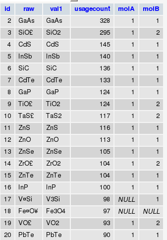
The information in molA and molB columns are populated from formulas using the following MySQL commands:
AB
UPDATE dbl014 SET molA=1, molB=1 WHERE val1 NOT REGEXP "[0-9]"
AB[0-9]
UPDATE `dbl014` SET molA=1 WHERE val1 NOT REGEXP "[0-9][A-Z]" AND molA IS NULL
A[0-9]B
UPDATE `dbl014` SET molB=1 WHERE val1 NOT REGEXP "[0-9]$" AND molB IS NULL
A2B
UPDATE `dbl014` SET molA=2 WHERE val1 REGEXP "[A-z]2[A-z]" AND molB =1
AB2
UPDATE `dbl014` SET molB=2 WHERE val1 REGEXP "[A-z]2$" AND molA =1
But we will be focusing only to the AB compositon today.
In addition, I have another table where I store information about elements:
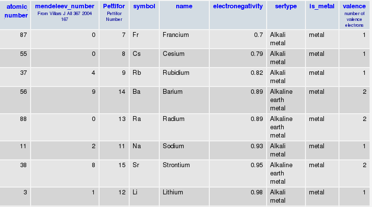
So I can go between Symbol to Atomic Number to Mendeleev Number as I please..
Here is what I did:
* Retrieved the complete list of AB compositions.
* Retrieved the reported structures and the temperature and pressure of the entries for each composition.
* Filtered the ones that weren’t measured/calculated at ambient pressure
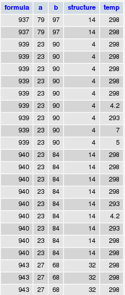
* Also recorded each component’s Mendeleev number, so at the end I obtained the following table where formula and structure information is enumerated (for instance, the values you see in the formula column are nothing but the ids of the formulas you can see in the first figure):
* Next, selected those that were measured in ambient temperature (something like SELECT * FROM db.table GROUP BY structure, formula WHERE temp=298)
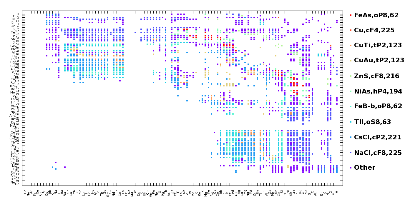
* Builded a histogram for structure populations, took the first 10 most populated structures as distinct and joining the rest as "other" (assigned structure number of "0"). By the way, here are the top 20 structures for AB compositions with the first number in parentheses showing its rank among binary compounds while the second is the number AB compositions registered in that structure type:
1 — NaCl,cF8,225 (4) (347)
2 — CsCl,cP2,221 (7) (306)
3 — TlI,oS8,63 (14) (126)
4 — FeB-b,oP8,62 (32) (69)
5 — NiAs,hP4,194 (16) (62)
6 — ZnS,cF8,216 (9) (51)
7 — CuAu,tP2,123 (44) (42)
8 — CuTi,tP2,123 (76) (34)
9 — Cu,cF4,225 (3) (34)
10 — FeAs,oP8,62 (51) (30)
11 — ZnO,hP4,186 (23) (28)
12 — W,cI2,229 (2) (26)
13 — FeSi,cP8,198 (57) (25)
14 — Mg,hP2,194 (5) (25)
15 — NaPb,tI64,142 (207) (14)
16 — ZrCl,hR12,166 (365) (14)
17 — NaO,hP12,189 (208) (13)
18 — AuCd,oP4,51 (121) (10)
19 — WC,hP2,187 (138) (10)
20 — DyAl,oP16,57 (149) (10)
* Wrote these data into a file ("str_wo_temp.txt" for further references) with [a] | [b] | [structure] being the columns as in :
79 100 11
26 93 11
24 93 11
73 92 11
78 100 11
27 64 0
66 92 0
12 97 0
53 101 0
61 86 4
31 84 4
23 85 4
32 85 4
33 85 4
27 85 4
so it was piece of a cake (not that easy, actually 8) to plot this using gnuplot :
set term wxt
set palette rgb 33,13,10
set view map
splot "str_wo_temp.txt" with points palette pt 5 ps 0.6
set xtics rotate by 90
set xtics("He" 1, "Ne " 2, "Ar" 3, "Kr " 4, "Xe" 5, "Rn " 6, "Fr" 7, "Cs " 8, "Rb" 9, "K " 10, "Na" 11, "Li " 12, "Ra" 13, "Ba " 14, "Sr" 15, "Ca " 16, "Yb" 17, "Eu " 18, "Sc" 19, "Lu " 20, "Tm" 21, "Er " 22, "Ho" 23, "Dy " 24, "Y" 25, "Tb " 26, "Gd" 27, "Sm " 28, "Pm" 29, "Nd " 30, "Pr" 31, "Ce " 32, "La" 33, "Lr " 34, "No" 35, "Md " 36, "Fm" 37, "Es " 38, "Cf" 39, "Bk " 40, "Cm" 41, "Am " 42, "Pu" 43, "Np " 44, "U" 45, "Pa " 46, "Th" 47, "Ac " 48, "Zr" 49, "Hf " 50, "Ti" 51, "Ta " 52, "Nb" 53, "V " 54, "W" 55, "Mo " 56, "Cr" 57, "Re " 58, "Tc" 59, "Mn " 60, "Fe" 61, "Ru " 62, "Os" 63, "Co " 64, "Rh" 65, "Ir " 66, "Ni" 67, "Pt " 68, "Pd" 69, "Au " 70, "Ag" 71, "Cu " 72, "Mg" 73, "Hg " 74, "Cd" 75, "Zn " 76, "Be" 77, "Tl " 78, "In" 79, "Al " 80, "Ga" 81, "Pb " 82, "Sn" 83, "Ge " 84, "Si" 85, "B " 86, "Bi" 87, "Sb " 88, "As" 89, "P " 90, "Po" 91, "Te " 92, "Se" 93, "S " 94, "C" 95, "At " 96, "I" 97, "Br " 98, "Cl" 99, "N " 100, "O" 101, "F " 102, "H" 103)
set ytics("He" 1, "Ne " 2, "Ar" 3, "Kr " 4, "Xe" 5, "Rn " 6, "Fr" 7, "Cs " 8, "Rb" 9, "K " 10, "Na" 11, "Li " 12, "Ra" 13, "Ba " 14, "Sr" 15, "Ca " 16, "Yb" 17, "Eu " 18, "Sc" 19, "Lu " 20, "Tm" 21, "Er " 22, "Ho" 23, "Dy " 24, "Y" 25, "Tb " 26, "Gd" 27, "Sm " 28, "Pm" 29, "Nd " 30, "Pr" 31, "Ce " 32, "La" 33, "Lr " 34, "No" 35, "Md " 36, "Fm" 37, "Es " 38, "Cf" 39, "Bk " 40, "Cm" 41, "Am " 42, "Pu" 43, "Np " 44, "U" 45, "Pa " 46, "Th" 47, "Ac " 48, "Zr" 49, "Hf " 50, "Ti" 51, "Ta " 52, "Nb" 53, "V " 54, "W" 55, "Mo " 56, "Cr" 57, "Re " 58, "Tc" 59, "Mn " 60, "Fe" 61, "Ru " 62, "Os" 63, "Co " 64, "Rh" 65, "Ir " 66, "Ni" 67, "Pt " 68, "Pd" 69, "Au " 70, "Ag" 71, "Cu " 72, "Mg" 73, "Hg " 74, "Cd" 75, "Zn " 76, "Be" 77, "Tl " 78, "In" 79, "Al " 80, "Ga" 81, "Pb " 82, "Sn" 83, "Ge " 84, "Si" 85, "B " 86, "Bi" 87, "Sb " 88, "As" 89, "P " 90, "Po" 91, "Te " 92, "Se" 93, "S " 94, "C" 95, "At " 96, "I" 97, "Br " 98, "Cl" 99, "N " 100, "O" 101, "F " 102, "H" 103)
set xtics font "Helvatica,8"
set ytics font "Helvatica,8"
set xrange [0:103]
set yrange [0:103]
#set term postscript enhanced color
#set output "pettifor.ps"
replot
and voila (or the real one with the accent which I couldn’t manage to 8) ! So here is the updated Pettifor Map for you (and for the AB compositons 8) But mind you, it doesn’t contain possible entries after year 2000.
You can plot the "same" map with Octave somewhat as follows (since I’m a newbie in Octave myself, I’ll take you as far as I could go – from there on, you’re on your own 8)
First, load the data file into a matrix:
load str_wo_temp.txt
then map this matrix contents into another matrix with the first (a) and second (b) columns being the new matrix’s column and row number and the third column (structure) being the value:
for i = 1:length(str_wo_temp)
A(str_wo_temp(i,1),str_wo_temp(i,2)) = str_wo_temp(i,3);
endfor
now, finally we can plot the density matrix:
imagesc(A)
which produces:
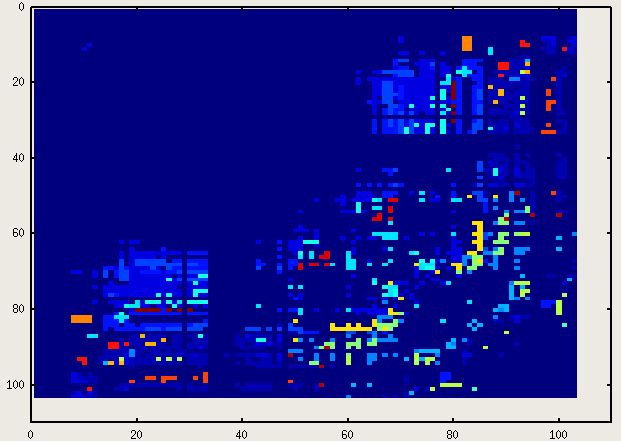
Oh, don’t be so picky about the labels and that thing called "legend"! 8) (By the way, if you know how to add those, please let me know, too – I haven’t started googling around the issue for the moment..)
While I was at it, I also plotted a 3-D Pettifor Map with the z-axis representing the temperature at which the structure was determined. This time, instead of saving all the data into one file, I saved the [a] [b] [temp] values into "structure name" files. Then, I picked up the most populated structure types (i.e., the ones contating the most lines) and moved the remaining into a temporary folder where I issued the
cat *.txt > others.txt
command. Then plotted this 3D map via gnuplot with the following command:
splot "NaCl,cF8,225.txt", "CsCl,cP2,221.txt", "TlI,oS8,63.txt", "FeB-b,oP8,62.txt", "NiAs,hP4,194.txt", "ZnS,cF8,216.txt", "FeAs,oP8,62.txt", "Cu,cF4,225.txt", "W,cI2,229.txt", "CuTi,tP2,123.txt", "CuAu,tP2,123.txt", "ZnO,hP4,186.txt", "Mg,hP2,194.txt", "FeSi,cP8,198.txt", "GeS,oP8,62.txt", "NaPb,tI64,142.txt", "AuCd,oP4,51.txt", "ZrCl,hR12,166.txt", "NaO,hP12,189.txt", "CuI,cF20,216.txt", "DyAl,oP16,57.txt", "InBi,tP4,129.txt", "PbO,tP4,129.txt", "CoO,tI4,139.txt", "WC,hP2,187.txt", "MoC,hP8,194.txt", "NaTl,cF16,227.txt", "GeTe,hR6,160.txt", "Sn,tI4,141.txt", "HgIn,hR6,166.txt", "In,tI2,139.txt", "PdBi,mP16,4.txt", "Nd,hP4,194.txt", "CuTi,tP4,129.txt", "NaP,oP16,19.txt", "HgS,hP6,152.txt", "CoSn,hP6,191.txt", "KGe,cP64,218.txt", "HgCl,tI8,139.txt", "AgI,cI38,229.txt", "others.txt"
Here are two snapshots:

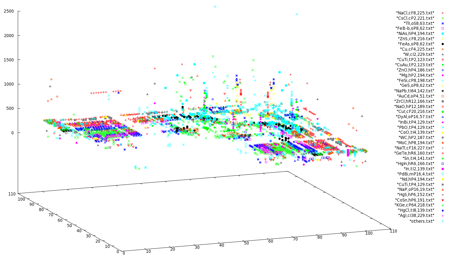
I’m planning to include a java version of this 3D map where you can more easily read what you are looking…
